
A replicable methodology for leveraging high-frequency building material indices as leading indicators of quarterly earnings
Using Building Products Transaction Data to Forecast Public Company Performance
March 12, 2026
I. Executive Summary
Building products transaction data—daily indices tracking price, quantity, and sales of lumber, OSB, plywood, gypsum, wallboard, and commercial gypsum—provides a powerful leading signal for predicting quarterly financial performance of publicly traded companies in the housing and construction ecosystem.
This paper describes a methodology that transforms daily, granular building material indices into quarterly predictive features, aligns them to company fiscal calendars, and fits an ensemble of four models (SARIMAX, Prophet, Elastic Net, and XGBoost) to forecast year-over-year changes in company KPIs such as revenue, volume, and comparable sales. The ensemble is weighted by inverse Mean Absolute Error, allowing the system to automatically favor the most accurate model for each company-KPI pair.
The approach exploits a fundamental asymmetry: building products transactions occur continuously, but the companies that depend on these materials report results only once per quarter. By the time a company announces earnings, the building products data has already observed the underlying demand conditions for weeks or months. Through lag optimization across 0–2 quarters, the system discovers these lead-lag relationships automatically, capturing the natural propagation delay from material transactions to corporate revenue recognition.
Key Finding: Building products indices lead company financial performance by 0–2 quarters. An inverse-MAE weighted ensemble of four models consistently improves upon both individual model predictions and analyst consensus estimates for companies with strong building material exposure.
II. Introduction: The Information Gap
Investors and analysts seeking to forecast the financial performance of building products companies, home improvement retailers, and homebuilders face a structural information disadvantage. Public company earnings are reported quarterly, typically 4–6 weeks after the period ends. Analyst consensus estimates rely on survey-based models, management guidance, and macroeconomic indicators—all of which are lagging or low-frequency by nature.
Meanwhile, the underlying building products market generates daily transaction data: every sheet of plywood, every board foot of lumber, every pallet of wallboard that moves through the distribution chain produces a data point. Aggregated and anonymized, these transactions form indices that reflect real-time demand conditions across the United States, broken down by product, geography, and metric type.
The central thesis of this methodology is straightforward: aggregate building material transaction flows are a leading indicator of financial performance for companies in the housing and construction value chain. A spike in lumber quantity sold nationally today will appear as revenue growth for lumber manufacturers and distributors next quarter. A decline in gypsum prices in the Southeast signals margin pressure for wallboard producers with regional exposure.
This paper describes how we operationalize this thesis—transforming raw daily indices into quarterly predictive features, selecting the most relevant signals for each company, and fitting an ensemble of complementary models to produce forecasts that can be compared directly against analyst consensus.
III. The Building Products Dataset
Product Categories
The dataset covers six building product categories, spanning the two major material families used in residential and commercial construction:
| Category | Family | Primary Use |
|---|---|---|
| Lumber | Wood Products | Framing, structural |
| Plywood | Wood Products | Sheathing, subfloors |
| OSB (Oriented Strand Board) | Wood Products | Sheathing, roofing decks |
| Gypsum | Gypsum Products | Broad category |
| Wallboard | Gypsum Products | Interior walls, ceilings |
| Commercial Gypsum | Gypsum Products | Exterior siding, roofs |
Three Index Types
Each product category is tracked through three complementary indices that decompose market activity into distinct economic signals:
- Price Index — A Laspeyres-style index tracking price changes within the category. Reflects pricing power and cost inflation.
- Quantity Index — Tracks total units sold. Reflects real demand independent of price movements.
- Sales Index — Tracks total dollar sales (price × quantity). Reflects overall market size and revenue potential.
Why three indices matter: A company can grow revenue through higher prices (price index up, quantity flat), higher volume (quantity up, price flat), or both. Decomposing the signal lets the model distinguish between price-driven and volume-driven growth—a critical distinction for margins and sustainability.
Geographic Coverage
Data is available at four geographic tiers, following the U.S. Census Bureau hierarchy:
| Tier | Count | Examples |
|---|---|---|
| National | 1 | United States aggregate |
| Census Region | 4 | Northeast, Midwest, South, West |
| Census Division | 8 | South Atlantic, Pacific, Mountain, etc. |
| State | Variable | Subject to anonymization thresholds |
The combination of 6 products × 3 metrics × 13+ geographies produces over 200 individual time series, each updated daily. This breadth is a key advantage: it allows the modeling system to discover which specific product-geography-metric combination best predicts each company’s KPI, rather than relying on a single national aggregate.
Applicable Companies
This methodology is applicable to any publicly traded company with meaningful revenue exposure to building products—including lumber and wood panel manufacturers, gypsum and wallboard producers, building materials distributors, home improvement retailers, insulation installers, and homebuilders. The key requirement is that the company’s financial performance is influenced by the volume and pricing of building materials flowing through the distribution chain.
For each target company, the analyst should identify which product categories are most relevant to its business (e.g., wood products for a lumber manufacturer, gypsum products for a wallboard company) and ensure sufficient historical KPI data is available—a minimum of 8 quarters (2 years) of reported actuals is recommended for reliable model fitting.
IV. Methodology
4.1 Data Preparation
Raw daily index values must be transformed before they can serve as predictive features for quarterly company KPIs. The transformation pipeline has three stages: smoothing, year-over-year normalization, and quarterly alignment.
Rolling Window Smoothing
Daily index values contain substantial noise. A 91-day (approximately one quarter) rolling average is applied to each series, producing a smoothed signal that captures the underlying trend while filtering out day-to-day volatility:
Rolling Averaget = mean( Daily Valuest−90 … Daily Valuest )
The 91-day window was chosen deliberately: it approximates one fiscal quarter, which creates natural temporal alignment with the company KPI data we aim to predict. Alternative windows (30, 60, 182, 365 days) are available for different analytical purposes, but 91 days is the default for predictive modeling.
Year-over-Year Transformation
Absolute index levels differ across products and geographies, making cross-series comparison meaningless. Year-over-year (YoY) percentage change normalizes all series to a common scale and removes seasonality:
YoY Changet = ( Rolling Avgt − Rolling Avgt−365 ) / Rolling Avgt−365 × 100
This transformation has a 456-day warmup period (91-day window + 365-day lookback) before the first valid YoY value can be computed. All earlier values are set to NaN to ensure only statistically reliable comparisons are used.
Applying YoY to Company KPIs
Company KPI data must undergo the same YoY transformation so that both sides of the model speak the same language. Rather than predicting a company’s raw quarterly revenue (e.g., $38 billion), the model predicts its year-over-year percentage change (e.g., +5.6%).
The calculation is straightforward: compare each quarter to the same quarter one year earlier. If Home Depot reported $38B in Q1 2025 and $36B in Q1 2024, the KPI value used in the model is +5.6%. On quarterly data, this is computed as a 4-period percentage change—looking back 4 quarters (one full year)—which automatically compares Q1 to Q1, Q2 to Q2, and so on, eliminating seasonal effects.
KPI YoYQ1 2025 = ( ActualQ1 2025 − ActualQ1 2024 ) / ActualQ1 2024 × 100
This ensures both the target variable (company KPI) and the predictive features (BP indices) are expressed in identical units: percentage points of year-over-year growth. A model can meaningfully learn that “+8% YoY growth in national lumber prices predicts +5% YoY growth in lumber manufacturer revenue”—a relationship that would be impossible to express if the two sides were in different units.
Quarterly Alignment
Company financial results are reported on specific period-end dates dictated by their fiscal calendar. To align daily BP data to these quarterly anchor points, the system:
- Computes the 91-day rolling average on the full daily series
- Identifies the intersection of daily BP dates with company period-end dates
- Extracts rolling values only on those quarter-end dates
This produces a quarterly-frequency BP series that is precisely time-aligned with each company’s financial reporting. The alignment respects fiscal calendar diversity—Home Depot’s retail calendar (quarters ending January, April, July, October) produces different anchor dates than Boise Cascade’s standard calendar (March, June, September, December).
4.2 Feature Engineering
With over 200 individual BP time series available, selecting the right predictive features is critical. The feature engineering pipeline uses a three-stage funnel: correlation scanning, lag optimization, and top-N selection.
Correlation Scanning
For each company-KPI pair, Pearson correlations are computed between the company’s KPI YoY series and every available BP index YoY series (spanning all products, geographies, and metrics). The correlations are ranked by absolute value, and the top 10 are advanced to the next stage.
This broad scan is essential because it allows unexpected signals to emerge. A gypsum manufacturer might correlate most strongly with lumber quantity (a proxy for new construction starts) rather than gypsum price. A retailer’s revenue might track regional plywood demand in the South Atlantic more closely than any national aggregate.
Lag Optimization
Building products transactions don’t necessarily predict company results in the same quarter—supply chain delays, inventory cycles, and revenue recognition timing create natural lags. The lag optimization step tests three temporal alignments for each feature:
- Lag 0: Same quarter — BP activity and company results are contemporaneous
- Lag 1: BP leads by one quarter — material demand today predicts revenue next quarter
- Lag 2: BP leads by two quarters — longer supply chain or project pipeline delay
For each feature, the lag with the highest absolute correlation is selected. The resulting “lag-optimized” features capture the true predictive lead time between building material activity and financial outcomes.
Top-3 Feature Selection
After lag optimization, the three features with the strongest correlations are selected as exogenous regressors for all four models. Limiting to three features is deliberate: with typical sample sizes of 20–40 quarters, more features risk overfitting. Three features provide enough signal diversity while keeping the feature-to-observation ratio manageable.
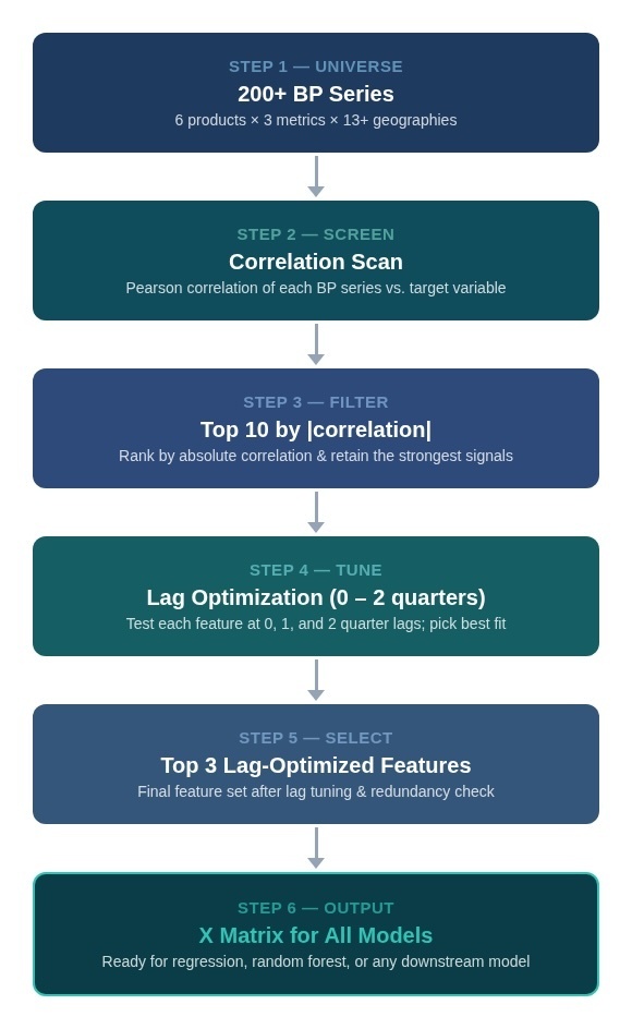
Figure 1: Feature selection funnel — from 200+ candidates to 3 lag-optimized predictors
4.3 Model Suite
The system fits four complementary models, each bringing different strengths to the prediction task. All four receive the same inputs: the company KPI YoY series as the target variable (y) and the three lag-optimized BP features as exogenous regressors (X).
SARIMAX
Seasonal ARIMA with eXogenous regressors. Captures temporal autocorrelation (last quarter predicts this quarter) and 4-quarter seasonality, while using BP features as external drivers.
Configuration: AR(1), seasonal AR(1) at lag 4, no differencing.
Strength: Explicitly models time-series structure.
Prophet
Facebook’s decomposable time-series model. Separates trend and yearly seasonality, with BP features added as linear regressors.
Configuration: Yearly seasonality on, weekly/daily off.
Strength: Robust to missing data, flexible seasonality.
Elastic Net
Regularized linear regression with blended L1 (Lasso) and L2 (Ridge) penalties. Automatically selects regularization strength via cross-validation.
Configuration: l1_ratio=0.5, 5-fold CV.
Strength: Handles multicollinearity, interpretable coefficients.
XGBoost
Gradient boosted decision trees with conservative hyperparameters tuned for small samples. Captures non-linear relationships between BP features and KPI outcomes.
Configuration: 10 trees, max depth 2, learning rate 0.3.
Strength: Non-linear patterns, automatic feature interactions.
4.4 Ensemble Approach
Individual models have complementary blind spots: SARIMAX can be too rigid if the relationship is non-linear; XGBoost can overfit with few observations; Prophet may over-model seasonality; Elastic Net may miss temporal dynamics. An ensemble that combines all four mitigates these individual weaknesses.
The ensemble uses inverse-MAE weighting: each model’s weight is proportional to the inverse of its Mean Absolute Error on the fitted data. Models with lower error receive higher weight; models that fail to fit are automatically excluded.
Weighti = (1 / MAEi) / ∑(1 / MAEj)
Ensemblet = ∑ Weighti × Predictioni,t
This approach is preferable to equal weighting because model accuracy varies significantly across companies. SARIMAX might dominate for a company with strong seasonal patterns, while Elastic Net might perform best for a company with a simple linear relationship to lumber prices. The inverse-MAE weighting discovers these preferences automatically.
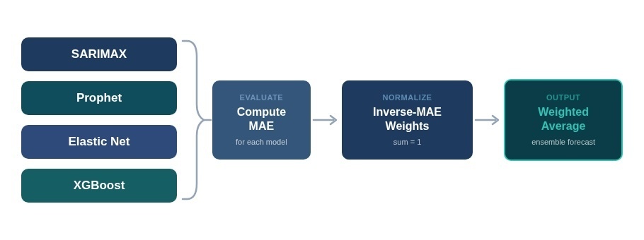
Figure 2: Ensemble construction — four models weighted by inverse MAE
V. Why Building Products Data Works as a Predictor
The predictive power of building products transaction data is not accidental. It arises from several structural properties of the housing and construction supply chain.
5.1 Demand Signals Precede Revenue Recognition
When a contractor purchases lumber for a framing job, that transaction appears in the building products data immediately. The revenue impact on the lumber manufacturer, however, may not be recognized until the following quarter—after the product ships, the invoice is processed, and the period closes. This timing gap creates a natural leading indicator: aggregate demand is observable in real time, but its financial consequences are reported with a lag.
The lag optimization step in our methodology quantifies this delay. For most companies, the optimal lag is 0–1 quarters, consistent with a typical 30–90 day pipeline from material purchase to revenue recognition. Some companies, particularly those further upstream (timberland REITs) or with longer project cycles, show optimal lags of 2 quarters.
5.2 Supply Chain Propagation
Building material demand propagates through the value chain in a predictable sequence. A housing start triggers demand for lumber (framing), then plywood and OSB (sheathing), then gypsum and wallboard (interior finishing). This sequential pattern means that changes in one product category can predict changes in another—and by extension, predict revenue for companies at different stages of the supply chain.
5.3 Geographic Granularity Captures Regional Exposure
National aggregates miss regional variation. A home improvement retailer with heavy exposure to the South Atlantic division will be more affected by construction activity in that region than by national trends. The building products dataset provides data at the regional and divisional level, allowing the modeling system to discover which geography best explains each company’s financial performance.
This is particularly valuable for companies with concentrated geographic footprints, or for detecting regional divergences that national data would obscure.
5.4 Price-Quantity-Sales Decomposition
The three-index structure (price, quantity, sales) provides richer signal than a single volume or revenue measure. Consider two scenarios:
- Prices up, quantity flat: Suggests cost inflation — may benefit commodity producers but squeeze distributor margins.
- Quantity up, prices down: Suggests strong demand but competitive pricing — volume-driven growth with margin pressure.
By testing all three index types during feature selection, the model can identify which decomposition best explains each company’s KPI. A lumber manufacturer’s revenue might correlate most strongly with lumber price (commodity exposure), while a distributor’s revenue correlates with lumber quantity (throughput-driven).
5.5 Daily Frequency Enables Responsive Smoothing
Unlike monthly or quarterly economic indicators (housing starts, building permits), the building products data is daily. This high frequency enables responsive rolling averages that detect trend changes within weeks rather than months. A 91-day rolling window captures the last quarter of activity; a sudden demand shift will begin moving the average within days, long before it appears in any government statistical release.
Key Insight: The building products dataset combines four properties rarely found together in alternative data: high frequency (daily), broad coverage (6 products, 13+ geographies), economic decomposition (price/quantity/sales), and direct connection to the end market (construction and renovation activity). This combination makes it a uniquely powerful leading indicator.
VI. Results and Evaluation
6.1 Choosing the Right Metrics
Model accuracy is measured using two complementary metrics: Mean Absolute Error (MAE) and R-squared (R²).
Why MAE, Not MAPE
Mean Absolute Percentage Error (MAPE) is a common accuracy metric but is poorly suited to YoY percentage data. When actual YoY values are near zero—which happens frequently during periods of flat growth—MAPE produces inflated, meaningless values. For example, an actual YoY of +1% with a prediction of +3% yields an APE of 200%, even though the absolute error is only 2 percentage points.
MAE, expressed in percentage points, directly measures the average magnitude of prediction errors:
MAE = mean( |Actuali − Predictedi| )
An MAE of 2.5pp means the model’s predictions are, on average, within 2.5 percentage points of the actual YoY change. This is intuitive and directly actionable.
| MAE Range | Assessment | Interpretation |
|---|---|---|
| < 3pp | Strong | Predictions typically within 3 percentage points of actual |
| 3 – 6pp | Moderate | Directionally useful; magnitude less precise |
| > 6pp | Weak | Limited predictive value for this company-KPI pair |
R-Squared for Explained Variance
R² measures the fraction of variance in the actual KPI series that the model explains:
R² = 1 − SSresidual / SStotal
An R² of 0.70 means the model explains 70% of the variation in quarterly YoY changes. Values above 0.5 generally indicate meaningful predictive power; values near or below zero indicate the model performs no better than predicting the historical average.
6.2 Ensemble vs. Consensus
The ensemble model can be compared directly against analyst consensus estimates, since both are expressed as predictions of the same target: quarterly KPI YoY change. Compute MAE and R² for both Consensus and Ensemble side by side to assess whether the building-products-enhanced model adds value beyond what the analyst community already captures.
The ensemble tends to outperform consensus in two scenarios:
- Commodity-exposed companies where building products prices directly drive revenue (e.g., lumber manufacturers). The BP data captures price movements that analysts may underweight or learn about with delay.
- Volume-driven inflections where construction activity shifts faster than analyst models update. The daily data detects demand changes weeks before they appear in housing starts or other macro releases that analysts monitor.
Consensus tends to outperform the ensemble when company performance is driven primarily by non-building-products factors (corporate actions, international operations, non-construction revenue streams).
6.3 Interpreting Ensemble Weights
The inverse-MAE weights reveal which modeling approach best fits each company. Inspecting these weights (e.g., SARIMAX: 35% | Prophet: 28% | Elastic Net: 22% | XGBoost: 15%) provides transparency into the ensemble’s composition.
Patterns in the weights can be informative:
- SARIMAX-dominated ensemble: Company KPI has strong temporal autocorrelation and seasonality. Past quarters are highly predictive of the current quarter.
- Elastic Net-dominated: Linear relationship between BP features and KPI. The signal is strong and direct.
- XGBoost-dominated: Non-linear or interaction-driven relationship. The company may respond differently to BP changes depending on the level (e.g., lumber price above a threshold triggers margin compression).
- Roughly equal weights: No single model has a clear edge; the ensemble is providing genuine diversification benefit.
VII. Best Practices and Limitations
7.1 Best Practices
Fiscal Calendar Alignment is Critical
The 14 tracked companies span three fiscal calendar types: standard (calendar year quarters), retail (4-5-4 week periods), and offset (fiscal year misaligned with calendar year). Misaligning BP data to the wrong period-end date introduces systematic error. The system uses company-reported period-end dates as the canonical temporal anchor, with configurable fiscal year and quarter offsets as fallback.
Use YoY, Not Sequential Quarter Growth
Sequential quarter-over-quarter growth is contaminated by seasonality (Q4 holiday spending, Q1 winter slowdowns). Year-over-year change eliminates seasonal effects and is the standard framework used by analysts for earnings comparisons. Both the BP features and the KPI targets should be expressed as YoY percentage change.
Limit Features to Avoid Overfitting
With typical sample sizes of 20–40 quarters, the ratio of observations to features is inherently low. Restricting to three exogenous features keeps the feature-to-observation ratio above 6:1, reducing overfitting risk. The regularized models (Elastic Net, conservative XGBoost) provide additional protection.
Let Lag Optimization Discover Lead Times
Do not assume a fixed lag for all companies. A lumber producer experiences demand contemporaneously (lag 0), while a home improvement retailer may see the impact one quarter later as consumer renovation projects complete (lag 1). The automatic lag optimization discovers these relationships from the data.
7.2 Limitations
Small Sample Sizes
Quarterly data limits sample sizes to approximately 20–40 observations per company. This constrains model complexity and statistical significance. The minimum sample threshold of 8 quarters is enforced, but even above this threshold, results should be interpreted with appropriate caution.
Signal Breakdown Scenarios
The predictive relationship between building products data and company performance can break down in specific circumstances:
- Supply shocks: Tariffs, natural disasters, or production outages can cause BP index spikes unrelated to demand.
- M&A activity: Acquisitions or divestitures change a company’s revenue composition, invalidating historical correlations.
- Revenue mix shifts: Companies diversifying away from building products reduce the predictive power of BP indices over time.
- Inventory cycles: Channel destocking or restocking can decouple transaction volumes from end demand.
Important: The building products model is one input among many. It excels at capturing demand-side signals that other data sources miss, but it should be used alongside—not as a replacement for—fundamental analysis, management guidance, and macroeconomic context.
Geographic Limitations
State-level data is not universally available due to anonymization requirements—states with low building products sales volumes or too few reporting entities are excluded. This limits the model’s ability to capture hyper-local demand patterns, particularly in smaller or less-developed markets.
VIII. Conclusion
Building products transaction data offers a unique and underutilized window into the real-time demand conditions that drive financial performance across the housing and construction ecosystem. By transforming daily indices into quarterly predictive features, aligning them to company fiscal calendars, and fitting an ensemble of four complementary models, we can produce forecasts that capture demand signals invisible to traditional analysis.
The methodology described in this paper can be applied to any publicly traded company with meaningful exposure to the housing and construction ecosystem. For each company, select the relevant KPIs, identify the most correlated building products indices, compare model performance against analyst consensus, and inspect ensemble weights and period-by-period accuracy.
Three principles underpin the approach:
- Let the data speak. Automatic correlation scanning and lag optimization discover predictive relationships rather than imposing assumptions.
- Ensemble for robustness. Four models with different structural assumptions, weighted by demonstrated accuracy, outperform any individual model on average.
- Transparency over black boxes. Every model’s MAE, R², and ensemble weight is visible. Users can assess confidence and identify when the signal is strong versus weak.
This document and its contents are the proprietary intellectual property of Rushmore Labs, LLC. No part of this publication may be reproduced, distributed, or transmitted in any form without the prior written permission of Rushmore Labs, LLC. All data is aggregated and anonymized. No individual company transaction data is disclosed.
Prepared by Jon Liggett, Head of Data Partnerships
With over 20 years of experience in investing and technology, Jon specializes in developing and promoting innovative data solutions that provide actionable business insights for leading brands.
How can we support your business?
Request to speak with a Rushmore Labs representative about your data needs.